# init repo notebook
!git clone https://github.com/rramosp/ppdl.git > /dev/null 2> /dev/null
!mv -n ppdl/content/init.py ppdl/content/local . 2> /dev/null
!pip install -r ppdl/content/requirements.txt > /dev/null

Bayes theorem continuous

import numpy as np
import matplotlib.pyplot as plt
from scipy import stats
from scipy.integrate import quad
from rlxutils import subplots, copy_func
from progressbar import progressbar as pbar
%matplotlib inline

def get_posterior(likelihood_fn, prior_fn, support, atol=1e-5, integration_intervals=1000):
    assert len(support)==2

    xr = np.linspace(*support, integration_intervals)

    Z = np.sum([likelihood_fn(x)*prior_fn(x) for x in xr]) * (xr[1]-xr[0])
    
    posterior_fn = lambda x: copy_func(likelihood_fn)(x) * copy_func(prior_fn)(x) /  Z
    
    return posterior_fn

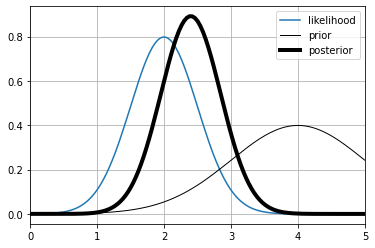
the posterior of one measurement

support = [-20,20]

likelihood = lambda x: stats.norm(loc=2,scale=.5).pdf(x)
prior      = lambda x: stats.norm(loc=4,scale=1).pdf(x)
posterior  = get_posterior(likelihood, prior, support)

xr = np.linspace(*support,1000)
plt.plot(xr, likelihood(xr), label="likelihood")
plt.plot(xr, prior(xr), label="prior", color="black", lw=1)
plt.plot(xr, posterior(xr), label="posterior", color="black", lw=4)
plt.grid();
plt.legend();
plt.xlim(0,5);

several measurements

we repeat the steps above, using the posterior obtained at each step as the prior for next measurement

def estimate_position(
    z_real = 23,
    prior_mean = 20,
    prior_std = 10,
    sensor_sigma = .7,
    support = [-10, 50]
):
    
    initial_prior      = eval(f"lambda x: stats.norm(loc={prior_mean},scale={prior_std}).pdf(x)")
    measurements = np.random.normal(loc=z_real, scale=sensor_sigma, size=10)
    posteriors = []
    
    prior = initial_prior
    for i in pbar(range(len(measurements))):
        # compute the likelihood
        likelihood = eval(f"lambda x: stats.norm(loc={measurements[i]},scale={sensor_sigma}).pdf(x)")
        
        # compute the posterior, stop if integration errors
        posterior = get_posterior(likelihood, prior, support)
        posteriors.append(posterior)

        # the posterior becomes the next prior 
        prior = posteriors[-1]
        
    # plot stuff
    xr = np.linspace(*support, 10000)
    for ax,i in subplots(len(posteriors)+1, n_cols=6):
        if i==0:
            plt.plot(xr, initial_prior(xr), color="steelblue")
            plt.title("prior")
            plt.ylim(0,0.5)
            plt.xlim(z_real-5, z_real+5)
        else:
            plt.plot(xr, posteriors[i-1](xr), color="steelblue")
            plt.title(f"measurement {i}")
            plt.axvline(measurements[i-1], color="black", ls="--")
            plt.xlim(z_real-2, z_real+2)

        plt.grid();
        plt.axvline(z_real, color="black")
    plt.tight_layout()

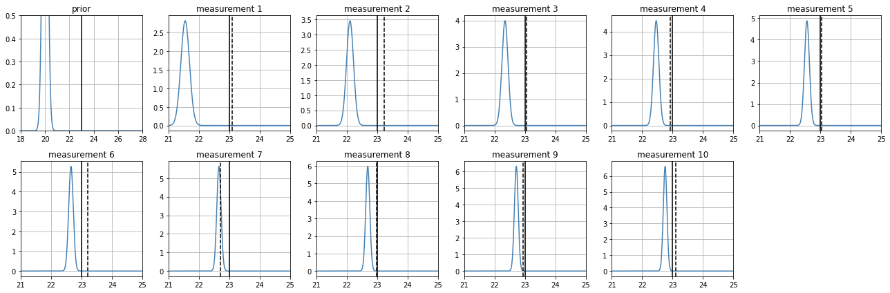
a very uninformative prior

observe how, as measurements are processed, the posterior becomes narrower (less uncertainty) and approaches the real value

estimate_position(
    z_real = 23,
    prior_mean = 5,
    prior_std = 20,
    sensor_sigma = .7
)

100% (10 of 10) |########################| Elapsed Time: 0:00:27 Time:  0:00:27

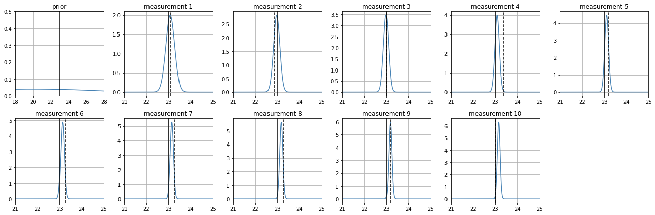
a more accurate sensor converges faster and with less ucertainty

however observe that numerical integration might stop us from processing further measurements

estimate_position(
    z_real = 23,
    prior_mean = 20,
    prior_std = 10,
    sensor_sigma = .2
)

100% (10 of 10) |########################| Elapsed Time: 0:00:28 Time:  0:00:28

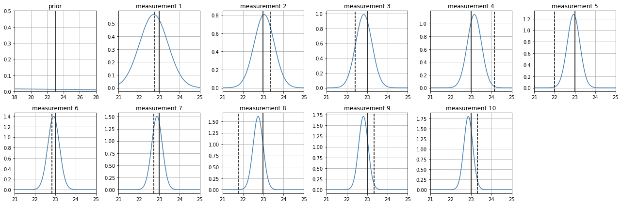
but if we are very wrong and very confident on our prior, we pay for it

Wrong mean with a very narrow stdev. It takes many measurements to converge to the real value.

Recall, narrow stdevs anywhere always represent small uncertainty

estimate_position(
    z_real = 23,
    prior_mean = 20,
    prior_std = .2,
    sensor_sigma = .2
)

100% (10 of 10) |########################| Elapsed Time: 0:00:28 Time:  0:00:28